Usage
Below are some examples of using the functions in Regressors package. The Boston data set will be used for demonstration purposes:
import numpy as np
from sklearn import datasets
boston = datasets.load_boston()
which_betas = np.ones(13, dtype=bool)
which_betas[3] = False  # Eliminate dummy variable
X = boston.data[:, which_betas]
y = boston.target
Obtaining Summary Statistics
There are several functions provided that compute various statistics about some of the regression models in scikit-learn. These functions are:
- regressors.stats.sse(clf, X, y)
- regressors.stats.adj_r2_score(clf, X, y)
- regressors.stats.coef_se(clf, X, y)
- regressors.stats.coef_tval(clf, X, y)
- regressors.stats.coef_pval(clf, X, y)
- regressors.stats.f_stat(clf, X, y)
- regressors.stats.residuals(clf, X, y)
- regressors.stats.summary(clf, X, y, Xlabels)
The last function, summary(), outputs the metrics seen above in a nice format.
An example with is developed below for a better understanding of these functions. Here, we use an ordinary least squares regression model, but another, such as Lasso, could be used.
SSE
To calculate the SSE:
from sklearn import linear_model
from regressors import stats
ols = linear_model.LinearRegression()
ols.fit(X, y)

stats.sse(ols, X, y)
Output:
11299.555410604258
Adjusted R-Squared
To calculate the adjusted R-squared:
from sklearn import linear_model
from regressors import stats
ols = linear_model.LinearRegression()
ols.fit(X, y)

stats.adj_r2_score(ols, X, y)
Output:
0.72903560136853518
Standard Error of Beta Coefficients
To calculate the standard error of beta coefficients:
from sklearn import linear_model
from regressors import stats
ols = linear_model.LinearRegression()
ols.fit(X, y)

stats.coef_se(ols, X, y)
Output:
array([  4.91564654e+00,   3.15831325e-02,   1.07052582e-02,
         5.58441441e-02,   3.59192651e+00,   2.72990186e-01,
         9.62874778e-03,   1.80529926e-01,   6.15688821e-02,
         1.05459120e-03,   8.89940838e-02,   1.12619897e-03,
         4.21280888e-02])
T-values of Beta Coefficients
To calculate the t-values beta coefficients:
from sklearn import linear_model
from regressors import stats
ols = linear_model.LinearRegression()
ols.fit(X, y)

stats.coef_tval(ols, X, y)
Output:
array([  7.51173468,  -3.55339694,   4.39272142,   0.72781367,
        -4.84335873,  14.08541122,   0.29566133,  -8.22887   ,
         5.32566707, -13.03948192, -11.14380943,   8.72558338,
        -12.69733326])
P-values of Beta Coefficients
To calculate the p-values of beta coefficients:
from sklearn import linear_model
from regressors import stats
ols = linear_model.LinearRegression()
ols.fit(X, y)

stats.coef_pval(ols, X, y)
Output:
array([  2.66897615e-13,   4.15972994e-04,   1.36473287e-05,
         4.67064962e-01,   1.70032518e-06,   0.00000000e+00,
         7.67610259e-01,   1.55431223e-15,   1.51691918e-07,
         0.00000000e+00,   0.00000000e+00,   0.00000000e+00,
         0.00000000e+00])
F-statistic
To calculate the F-statistic of beta coefficients:
from sklearn import linear_model
from regressors import stats
ols = linear_model.LinearRegression()
ols.fit(X, y)

stats.f_stat(ols, X, y)
Output:
114.22612261689403
Summary
The summary statistic table calls many of the stats outputs the statistics in an pretty format, similar to that seen in R.
The coefficients can be labeled more descriptively by passing in a list of lables. If no labels are provided, they will be generated in the format x1, x2, x3, etc.
To obtain the summary table:
from sklearn import linear_model
from regressors import stats
ols = linear_model.LinearRegression()
ols.fit(X, y)

xlabels = boston.feature_names[which_betas]
stats.summary(ols, X, y, xlabels)
Output:
Residuals:
     Min      1Q  Median      3Q      Max
-26.3743 -1.9207  0.6648  2.8112  13.3794


Coefficients:
             Estimate  Std. Error  t value   p value
_intercept  36.925033    4.915647   7.5117  0.000000
CRIM        -0.112227    0.031583  -3.5534  0.000416
ZN           0.047025    0.010705   4.3927  0.000014
INDUS        0.040644    0.055844   0.7278  0.467065
NOX        -17.396989    3.591927  -4.8434  0.000002
RM           3.845179    0.272990  14.0854  0.000000
AGE          0.002847    0.009629   0.2957  0.767610
DIS         -1.485557    0.180530  -8.2289  0.000000
RAD          0.327895    0.061569   5.3257  0.000000
TAX         -0.013751    0.001055 -13.0395  0.000000
PTRATIO     -0.991733    0.088994 -11.1438  0.000000
B            0.009827    0.001126   8.7256  0.000000
LSTAT       -0.534914    0.042128 -12.6973  0.000000
---
R-squared:  0.73547,    Adjusted R-squared:  0.72904
F-statistic: 114.23 on 12 features
Plotting
Several functions are provided to quickly and easily make plots useful for judging a model.
- regressors.plots.plot_residuals(clf, X, y, r_type, figsize)
- regressors.plots.plot_qq(clf, X, y, figsize)
- regressors.plots.plot_pca_pairs(clf_pca, x_train, y, n_components, diag, cmap, figsize)
- regressors.plots.plot_scree(clf_pca, xlim, ylim, required_var, figsize)
We will continue using the Boston data set referenced above.
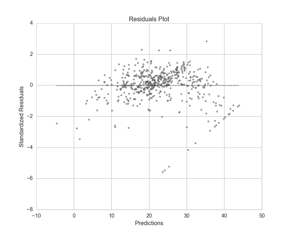
Residuals
Residuals can be plotted as actual residuals, standard residuals, or studentized residuals:
from sklearn import linear_model
from regressors import plots
ols = linear_model.LinearRegression()
ols.fit(X, y)

plots.plot_residuals(ols, X, y, r_type='standardized')
Plots:
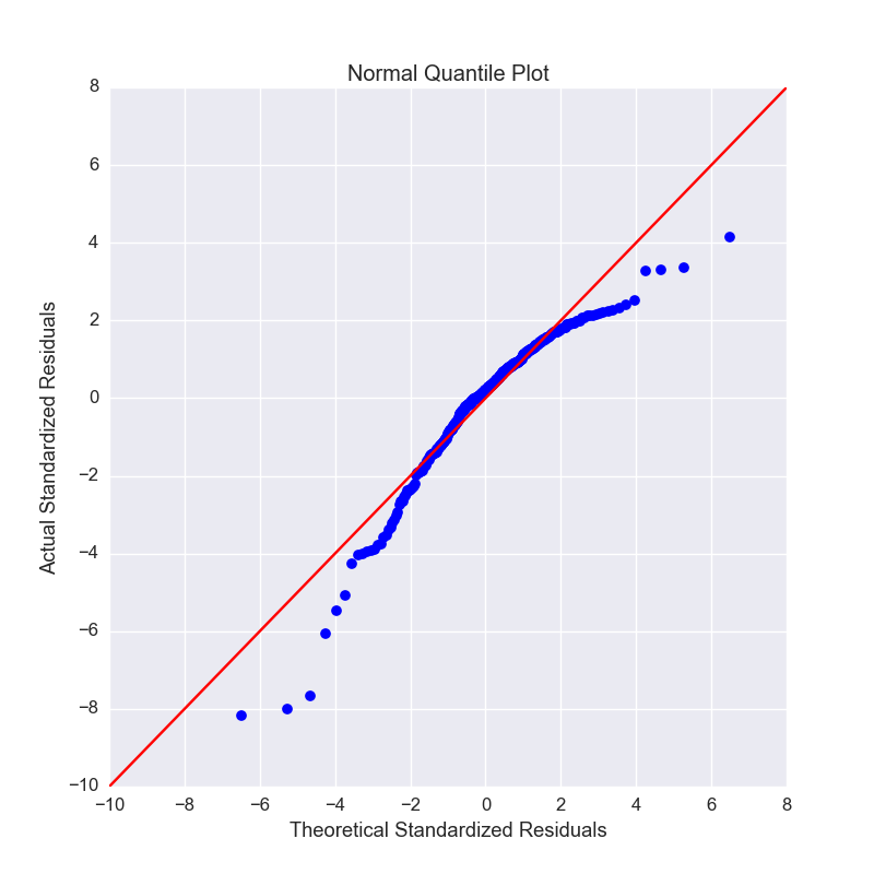
Q-Q Plot
Q-Q plots can quickly be obtained to aid in checking the normal assumption:
from sklearn import linear_model
from regressors import plots
ols = linear_model.LinearRegression()
ols.fit(X, y)

plots.plot_qq(ols, X, y, figsize=(8, 8))
Plots:
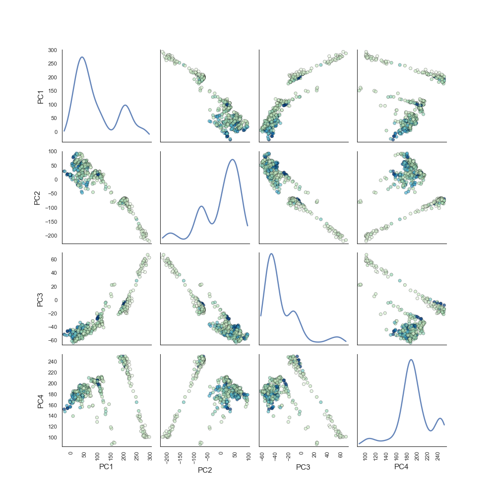
Principal Components Pairs
To generate a pairwise plot of principal components:
from sklearn import preprocessing
from sklearn import decomposition
from regressors import plots
scaler = preprocessing.StandardScaler()
x_scaled = scaler.fit_transform(X)
pcomp = decomposition.PCA()
pcomp.fit(x_scaled)

plots.plot_pca_pairs(pcomp, X, y, n_components=4, cmap="GnBu")
Plots:
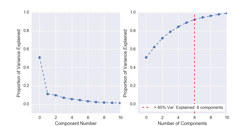
Scree Plot
Scree plots can be quickly generated to visualize the amount of variance represented by each principal component with a helpful marker to see where a threshold of variance is reached:
from sklearn import preprocessing
from sklearn import decomposition
from regressors import plots
scaler = preprocessing.StandardScaler()
x_scaled = scaler.fit_transform(X)
pcomp = decomposition.PCA()
pcomp.fit(x_scaled)

plots.plot_scree(pcomp, required_var=0.85)
Plots:
Principal Components Regression (PCR)
The PCR class can be used to quickly run PCR on a data set. This class
provides the familiar fit(), predict(), and score() methods that
are common to scikit-learn regression models. The type of scaler, the number
of components for PCA, and the regression model are all tunable.
PCR Class
An example of using the PCR class:
from regressors import regressors
pcr = regressors.PCR(n_components=10, regression_type='ols')
pcr.fit(X, y)

# The fitted scaler, pca, and scaler models can be accessed:
scaler, pca, regression = (pcr.scaler, pcr.prcomp, pcr.regression)

# You could then make various plots, such as pca_pairs_plot(), and
# plot_residuals() with these fitted model from PCR.
Beta Coefficients
The coefficients in PCR’s regression model are coefficients for the PCA space. To transform those components back to the space of the original X data:
from regressors import regressors
pcr = regressors.PCR(n_components=10, regression_type='ols')
pcr.fit(X, y)
pcr.beta_coef_
Output:
array([-0.96384079,  1.09565914,  0.27855742, -2.0139296 ,  2.69901773,
        0.08005632, -3.12506044,  2.85224741, -2.31531704, -2.14492552,
        0.89624424, -3.81608008])
Note that the intercept is the same for the X space and the PCA space, so
simply access that directly with pcr.self.regression.intercept_.